Population variance, sample variance and sampling variance

In finite population sampling context, the term variance can be confusing. One of the most common mistakes is mixing up population variance, sample variance and sampling variance. Some definitions may be helpful:

• Population variance \(S^2\): describes the variability of a characteristic in the population;
• Sample variance \(s^2\): describes the variability of a characteristic in the sample and can be used to estimate the population variance;
• Sampling variance \(Var( \overline{y} )\): describes the variability of estimates; in this case, the sample mean.

So, population variance is something that does not depend on the sampling method: if you use a SRS or cluster sample, that will not change the population variance of a characteristic. For example, consider the height: the variability of height in the population of adults is something that exists, no matter what sample you take.

Sample variance describes the variance of a characteristic in the sample. That can, indeed, be affected by the sample design. But, using the appropriate estimator, you can estimate the population variance of that characteristic using the variability that characteristic in the sample.

Sampling variance is something else. We have the population mean, \(\overline{Y}\). If we took a SRS sample from a population, we will have an estimate of \(\overline{Y}\), which we will call \(\overline{y}\). However, since many possible samples can be taken from a population, that estimate is only one in many possible estimates.

Let’s look at an example. Randomnopolis is a city with \(N = 100000\) habitants. This city is also a very careful place: every person alive has a record in the civil registration, such that it is possible to create a list of every person’s name, birth date, and address. The mayor asks the city’s statistician to estimate the mean of height, income and the proportion of short-sighted among the adults. However, he says he can only pay for \(n=1000\) interviews.

How many SRS¹ samples of \(n=1000\) individuals can be taken from a population of \(N=100000\) individuals? Well, it is a very large number: 1.7 \(\times\) (10 to the power 2430 ). Yes, we’re multiplying by an integer number that starts with 1 and is followed by 2430 zeroes. In fact, my computer cannot print this number: it simply says infinity.

\(1.7 \times 10^{2430}\) possible samples of \(10^3\) subjects… What were you saying about big data?

It would be nice to look at how the estimates \(\overline{y}\) are distributed across all possible samples. My computer can’t do that in my lifetime. But a statistician can! We know that those estimates have a normal distribution around the population mean, because the estimator of the sample mean is an unbiased estimator of the population mean. Besides, by knowing the distribution, the statistician can estimate an interval where we expect to see find the population total in 99% of all possible samples.

Let’s take this example a bit further. Suppose we are a magical being that knows the characteristics for each individual in the population. Here are the population characteristics:

##   height   income   myopic 
## 170.0098 721.1162   0.0506

This means that: the mean height of the population is 170 cm, the mean income is $ 196 and the proportion of short-sighted people is 5%, roughly speaking.

Besides, we can see all possible realities. But our computers are not that magical: we can process only 5000 out of those many realities. We then sample them and collect the results calculated by the statistician in those realities.

What is the average estimate for those samples?

## mean_height mean_income mean_myopic 
##    170.0122    721.3354      0.0505

On average, our statistician is doing a great job: the difference between the population mean and the mean of the estimates is quite small. Will any of them hit precisely the population mean? That is possible, but very unlikely. Does that mean that they are always wrong? Well, I’d rather say that – on average – they are correct.

Using the estimates of the sample mean and the sampling variance, they can estimate an interval where they are 99% confident to find the population mean. This is a tricky statement and is one of the most misunderstood sentences in statistics. We know that 99% of all possible samples would produce interval estimates containing the true parameter. To say we are 99% confident means that we are 99% sure that the particular sample we are working with is one of those. In Neyman’s words, if we repeated the sampling procedure many times, the confidence interval would contain the true value 99% of the time.

Let’s check if this is true with our sample of samples. The numbers below show how many of the 5000 confidence intervals contained the true population value of the mean for height, income and short-sightedness.

## [1] 0.991

## [1] 0.986

## [1] 0.988

Close enough, right?

And, since we can, let me show you the histogram of the population values:

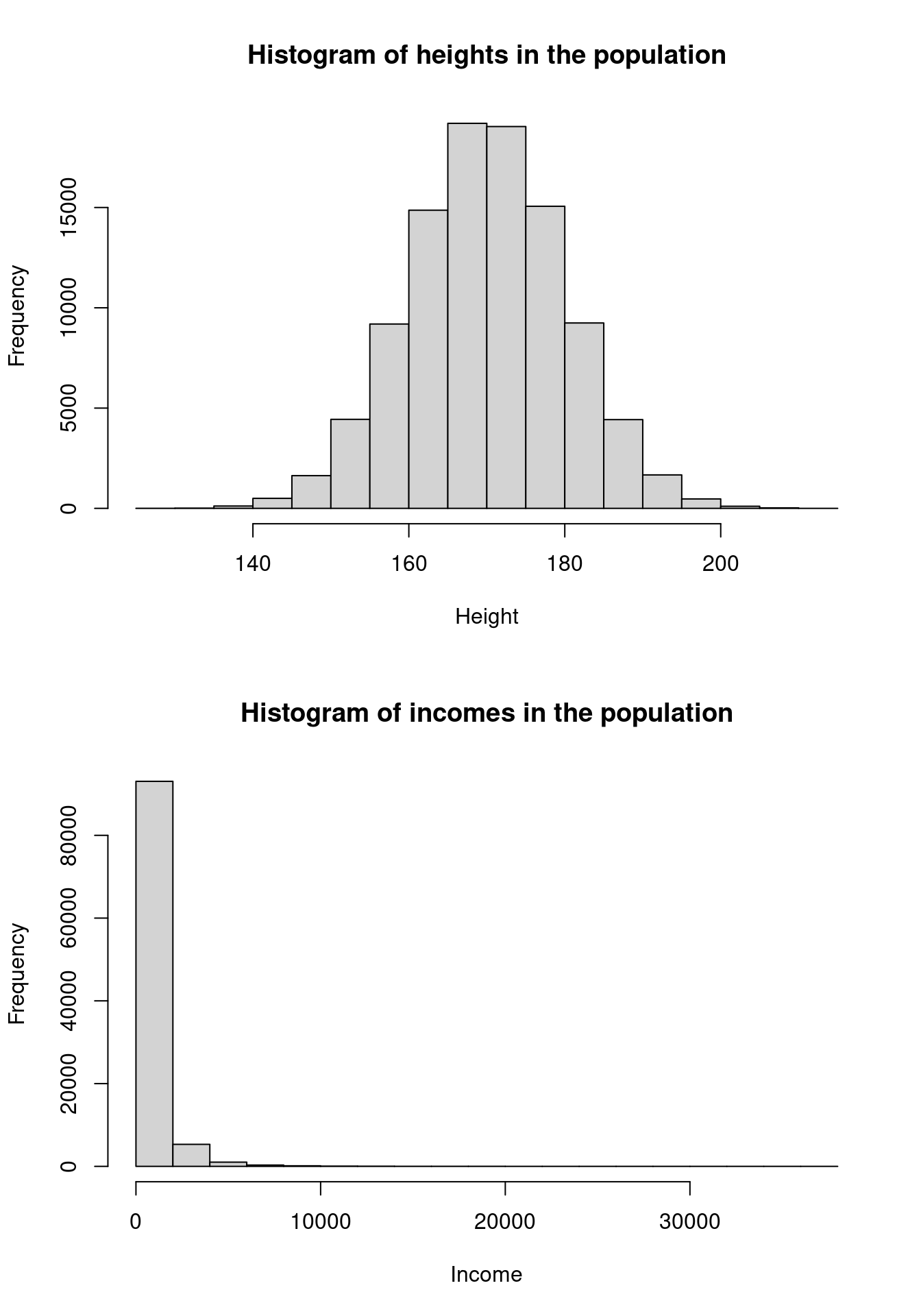
Now, look at the estimate distribution:

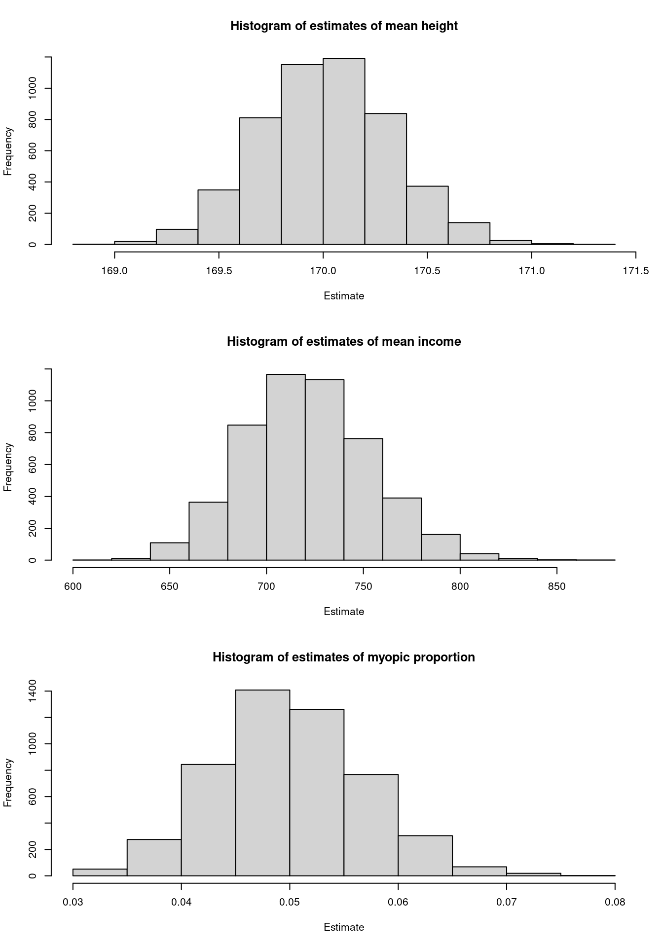
So, even when the population is not normally distributed, such as the income distribution, the sampling variance still works!